
Now available as a Python package! Install TurboQuant directly into your HuggingFace pipeline:
pip install turboquant-explainedimport turboquant cache = turboquant.patch_model(model, b_key=2, b_value=2)
2-bit keys + values = ~8x memory reduction with attention quality within ~2.7x of the Shannon limit. PyPI GitHub
Implementation Details
Overview
Key topics covered:
- MSE (Mean Square Error)
- Results / graphs
- Equations / math
- Potential datasets
2-Stage process:
- Stage 1 — MSE-optimal quantization
- Stage 2 — Inner-product correction via QJL residual
Datasets
| ID | Description | Link |
|---|---|---|
| D1 | DBpedia OpenAI embeddings — 1536-dim, 1M vectors | HuggingFace |
| D2 | DBpedia OpenAI embeddings — 3072-dim, 1M vectors | HuggingFace |
| D3 | GloVe 6B embeddings | Stanford |
| D4 | Needle in a Haystack benchmark | GitHub |
Models
| # | Model | Link |
|---|---|---|
| 1 | meta-llama/Llama-3.1-8B-Instruct (FP16) |
HuggingFace |
| 2 | bartowski/Meta-Llama-3.1-8B-Instruct-GGUF (quantized) |
HuggingFace |
Experimental Setup
Quantization targets: 2.5-bit and 3.5-bit
Following the experimental setup of Fu et al. [21], evaluations use the Llama-3.1-8B-Instruct model — a sweet spot between what was available, affordable, and convincing for an academic research paper.
Why Shannon’s Source Coding Entropy Matters
How much can you compress information without losing it — and what’s the absolute limit?
Shannon asked: given a budget of B bits, what’s the minimum distortion you can possibly achieve? The answer is the distortion-rate function D(B), and no algorithm can do better — ever.
TurboQuant’s distortion is within a factor of ~2.7 of Shannon’s theoretical limit. This means you physically cannot do much better regardless of how clever your algorithm is.
Core problem: LLMs are memory-bound, not compute-bound.
What Exactly Is Cached? (KV Cache)
The KV cache stores pre-computed Keys and Values for each past token.
- When generating token N, the model compares the current query against every previous token’s key, then weighted-sums their values.
- Without caching, K and V would be recomputed for all previous tokens at every single step.
- The KV cache saves those already-computed vectors to avoid recomputation.
KV Cache Memory Example
Llama 3.1 8B: 32 layers, 8 KV heads, head_dim = 128, FP16 = 2 bytes/float
Per token = layers × heads × 2 (K and V) × head_dim × bytes
           = 32 × 8 × 2 × 128 × 2 bytes
           = 131 KB / token

For 128K context = 131 KB × 131,072 ≈ 16 GB
Shannon Lower Bound (Lemma 3)
The absolute minimum distortion achievable given a specific bit budget:
D(B) ≥ 2^(−2B/d)
Where:
D(B)= minimum achievable distortion (MSE)B= total bit budgetd= dimension of the vector
Key insight: Double your bit budget (B → 2B) and the distortion drops by 4×. This is the fundamental compression–quality tradeoff — you pay exponentially in bits to gain linearly in quality.
Pipeline
vector → random rotation → Beta distribution (Lemma 1) → Gaussian (high-d) → scalar quantization
Stage 1: MSE-Optimal Quantization
Key idea: Store a high-dimensional vector into few bits while preserving the most important information.
Growing KV cache sizes in transformers make this critical — we need quantization that preserves both MSE and inner-product structure.
Distortion Metrics
MSE distortion — how close the reconstructed vector is to the original:
D_mse = E[ ||x − Q⁻¹(Q(x))||² ]
Inner-product distortion — how much quantization alters stored information:
D_prod = E[ |⟨y, x⟩ − ⟨y, Q⁻¹(Q(x))⟩|² ]
Nearest-neighbour / vector search using cosine similarity must remain intact after quantization.
Primitives:
Q— QuantizerQ⁻¹— DeQuantizer
Key Ideas
- Random rotation — makes any vector’s coordinates statistically predictable
- Scalar quantization per coordinate — enabled by near-independence after rotation
- Inner-product residual correction — QJL step restores unbiasedness
Stage 2: Why Random Rotation Helps
Consider a KV cache vector with all energy in one dimension:
x = [0.98, 0.02, 0.01, 0.003, …]
A naïve quantizer would need a different codebook per dimension. Most dimensions are near-zero, a few are high-value — this uneven energy distribution is hard to quantize uniformly.
Solution: Apply a random rotation generated from a random Gaussian matrix via QR decomposition to obtain an orthogonal matrix. This spreads energy evenly across all dimensions.
At d = 128 and above, after rotation we get:
- Beta distribution approximates Gaussian
- Near-independence between coordinates
- Concentrated, symmetric coordinate values
Lemma 1: Coordinate Distribution After Rotation
For a vector uniformly distributed on the unit hypersphere, each coordinate follows a Beta-related distribution:
f_X(x) = Γ(d/2) / (√π · Γ((d−1)/2)) · (1 − x²)^((d−3)/2)
Where:
f_X(x)is the probability density function (PDF)Γ(·)is the gamma function:Γ(n) = (n−1)!- The term
(1 − x²)^((d−3)/2)controls the shape
In high dimensions (d → ∞), this converges to N(0, 1/d).
Intuition: 3D Sphere Example
For a 3D sphere (d = 3): (1 − x²)^((3−3)/2) = (1 − x²)^0 = 1
The density is flat on [−1, 1] — one coordinate of a 3D unit sphere is uniformly distributed.
Think of the Earth:
- Fix the z-axis (latitude)
- At any latitude, the remaining coordinates lie on a circle
- Poles → small circle (low probability)
- Equator → large circle (higher probability)
Why Gaussian Properties Are Valuable
| Property | Benefit |
|---|---|
| Symmetry around 0 | Simple codebook; few parameters needed |
| Most values near 0 | Many small values → easy to compress |
| Few large values | Can tolerate larger error at the tails |
| Separable structure | Hard d-dimensional quantization → easy 1D quantization |
Stage 3 - TurboQuant-MSE (coarse quantization)
1. Rotate vector
y = Πx
2. Quantize each coordinate — find nearest centroid
yj → ck (argmin_k |yj - ck|)
3. Store centroid index
index_j = 2
4. Dequantize — lookup centroid value
ỹj = c[index_j]
5. Rotate back — reconstruct original space
x̃ = Πᵀ ỹ
Why Lloyl-Max is the right tool:
- How do we optimally quantize one scalar drawn from a known distribution?
- Find optimal quantization levels that minimize mean squared error (MSE)
Inputs:
- Probability distribution
- No. of quantization levels K
Outputs:
- Optimal thresholds
- Optimal reconstruction values
How are the optimal centroids determined (Lloyd-Max)
Minimize: Σ(x - c_i)² — iterate two steps until convergence:
- Assign each value to nearest centroid
- Update each centroid to mean of its assigned values
Example: 8 values → 4 centroids (2 bits)
Data:     [-0.95, -0.72, -0.61, -0.08,  0.12,  0.28,  0.76,  0.91]
c⁰:       [-0.8,  -0.2,   0.2,   0.8]

Assign → nearest centroid:
  {-0.95, -0.72, -0.61} → -0.8  |  {-0.08} → -0.2  |  {0.12, 0.28} → 0.2  |  {0.76, 0.91} → 0.8

Update → cluster means:
  c¹ = [-0.76, -0.08, 0.20, 0.835]   (assignments unchanged → converged)

Result:
  Original:   -0.95  -0.72  -0.61  -0.08   0.12   0.28   0.76   0.91
  Quantized:  -0.76  -0.76  -0.76  -0.08   0.20   0.20   0.84   0.84
Centroids are denser where data clusters — the quantizer adapts to the distribution.
Full TurboQuant-MSE Workflow
x → y = Πx → ỹ (Lloyd-Max quantized) → x̃ = Πᵀỹ
Example: x = [1, 0], 90° rotation matrix
Step 1 — Rotate:       Π = [[ 0, -1],    y = Π x = [0, 1]
                             [ 1,  0]]

Step 2 — Quantize:     y = [0, 1]  →  ỹ = [0.1, 0.9]   (Lloyd-Max centroids)

Step 3 — Rotate back:  Πᵀ = [[ 0, 1],   x̃ = Πᵀ ỹ = [0.9, -0.1]
                              [-1, 0]]
| x | y | ỹ | x̃ | |
|---|---|---|---|---|
| Values | [1, 0] | [0, 1] | [0.1, 0.9] | [0.9, −0.1] |
Original [1, 0] → reconstructed [0.9, −0.1] — close but slightly distorted. That’s quantization error.
Output : x~mse
Stage 4: Quantize Residual with 1-bit QJL (Fine Correction)
x → Q_mse(x) → r = x − x̃_mse → Q_qjl(r) → r̃ → x̃ = x̃_mse + r̃
The residual r = x − x̃_mse captures what MSE quantization missed. It gets 1-bit quantized via the QJL (Quantized Johnson-Lindenstrauss) transform.
Example:
x      = [ 1.0,  0.5, -0.2]
x̃_mse  = [ 0.9,  0.6, -0.3]
r      = [ 0.1, -0.1,  0.1]   ← residual to encode
Johnson-Lindenstrauss Trick
Q_qjl(r) = sign(S · r)
S ∈ ℝ^(d×d) is a random Gaussian matrix (S ~ N(0,1)) — projects r onto random directions, then takes the sign of each projection.
Step-by-step:
r = [0.2, -0.1, 0.05]

S = [[ 0.5, -1.2,  0.3],     # random Gaussian matrix
     [-0.7,  0.4,  1.1],
     [ 0.2, -0.9,  0.6]]

Sr = S · r = [ 0.235, -0.125, 0.160]   ← projections onto random directions

Q_qjl(r) = sign(Sr) = z = [+1, -1, +1]    ← 1 bit per dimension
Each coordinate compressed to a single bit: +1 if projection > 0, -1 if < 0.
Stage 5: Reconstruct Residual
Dequantize QJL:
Q_qjl⁻¹(z) = √(π/2) · (1/d) · Sᵀ · z
Sᵀ is the transpose of the same random matrix from Stage 4. The √(π/2) / d factor makes the estimator unbiased for inner products.
Example (continuing from Stage 4):
z  = [+1, -1, +1]

Sᵀ = [[ 0.5, -0.7,  0.2],
      [-1.2,  0.4, -0.9],
      [ 0.3,  1.1,  0.6]]

Sᵀ · z = [0.5+0.7+0.2,  -1.2-0.4-0.9,  0.3-1.1+0.6] = [1.4, -2.5, -0.2]
Scale by residual norm γ = ‖r‖₂ (stored during quantization):
γ = ‖[0.2, -0.1, 0.05]‖ = √(0.04 + 0.01 + 0.0025) ≈ 0.2291

r̃ = γ · √(π/2)/d · Sᵀz ≈ [0.134, -0.239, -0.019]
Comparison:
| dim 1 | dim 2 | dim 3 | |
|---|---|---|---|
| r (true) | 0.200 | −0.100 | 0.050 |
| r̃ (reconstructed) | 0.134 | −0.239 | −0.019 |
Not exact — and that’s expected. QJL uses only 1 bit per dimension and is designed for unbiased inner-product estimation, not coordinate-wise recovery. The residual correction fixes inner-product bias even though r̃ is a rough approximation of r.
Stage 6: Final reconstruction
Combine the MSE reconstruction with the QJL residual correction:
x̃ = x̃_mse + r̃
Example comparison:
| x₁ | x₂ | x₃ | |
|---|---|---|---|
| Original x | 1.0 | 0.5 | −0.2 |
| Stage 3 only x̃_mse | 0.9 | 0.6 | −0.3 |
| Stage 4 final x̃ | 1.034 | 0.361 | −0.319 |
Important note
Stage 4 does not always improve coordinate-wise accuracy. It improves:
- Inner product accuracy
- Unbiased estimation
- Geometric structure preservation
Other Key Ideas
| Idea | Description |
|---|---|
| Idea 1 | Random rotation makes any vector’s coordinates statistically predictable |
| Idea 2 | Lloyd-Max — optimal scalar quantization for a known distribution |
| Idea 3 | Why MSE quantizers are biased for inner products |
| Idea 4 | QJL — the residual fix that restores unbiasedness |
Simple Experiment: Verifying Lemma 1
- Draw
g ~ N(0, I₃) - Normalize:
x = g / ||g||₂ - Record the first coordinate
x₁ - Plot histogram → should be uniform on
[−1, 1]ford = 3
How Is the Rotation Matrix R Generated?
- Drawn randomly from a Gaussian distribution
- Must be orthogonal:
R Rᵀ = I - Method: QR decomposition of a random
N(0,1)matrix
Experimental Results
Math Validation
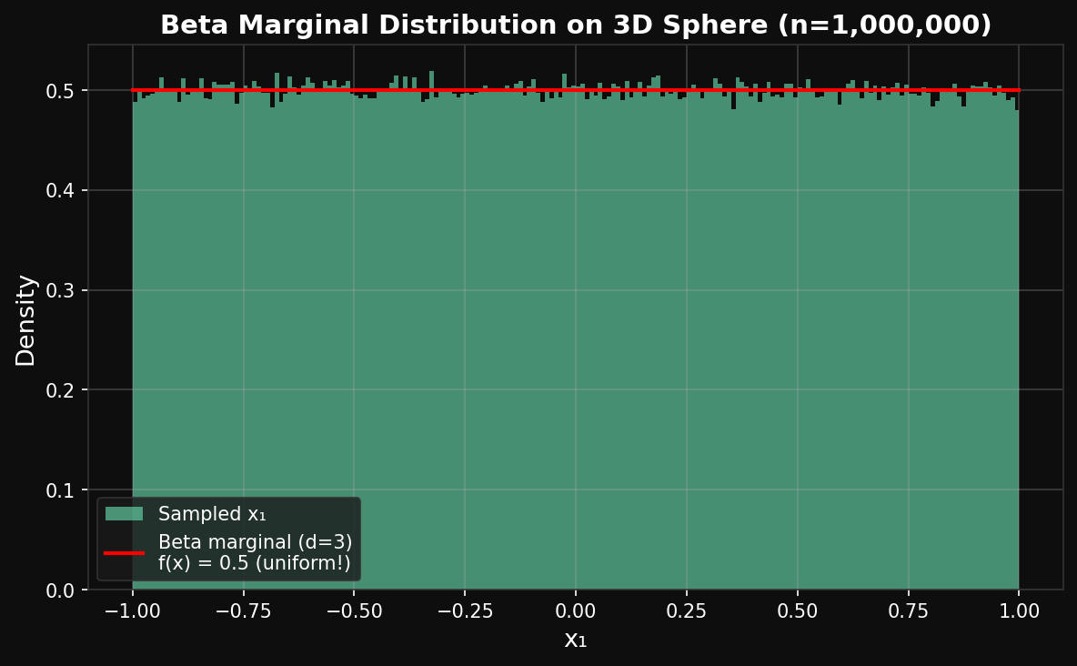 Beta marginal PDF for a single coordinate of a uniform random point on the 3D unit sphere (Lemma 1 verification).
Phase 1 — Synthetic Validation (d=1536)
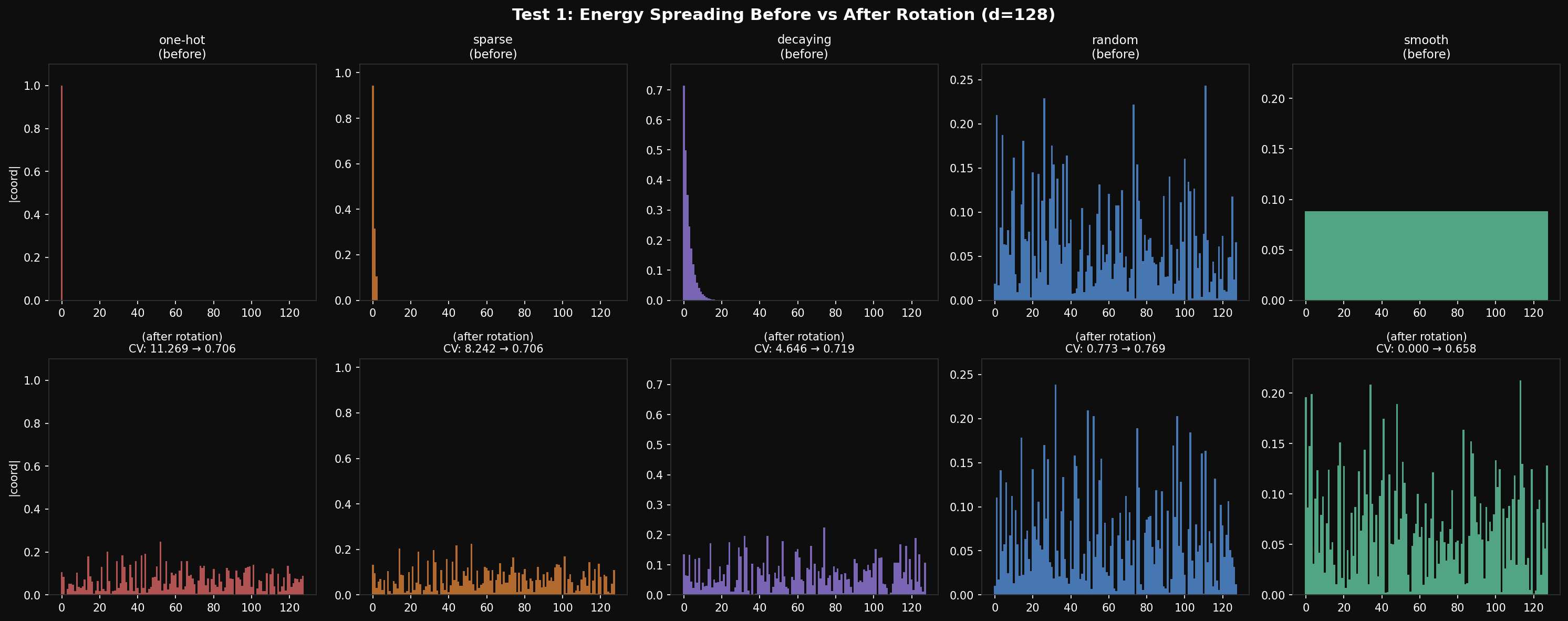 Random rotation spreads uneven energy across all coordinates, enabling uniform scalar quantization.
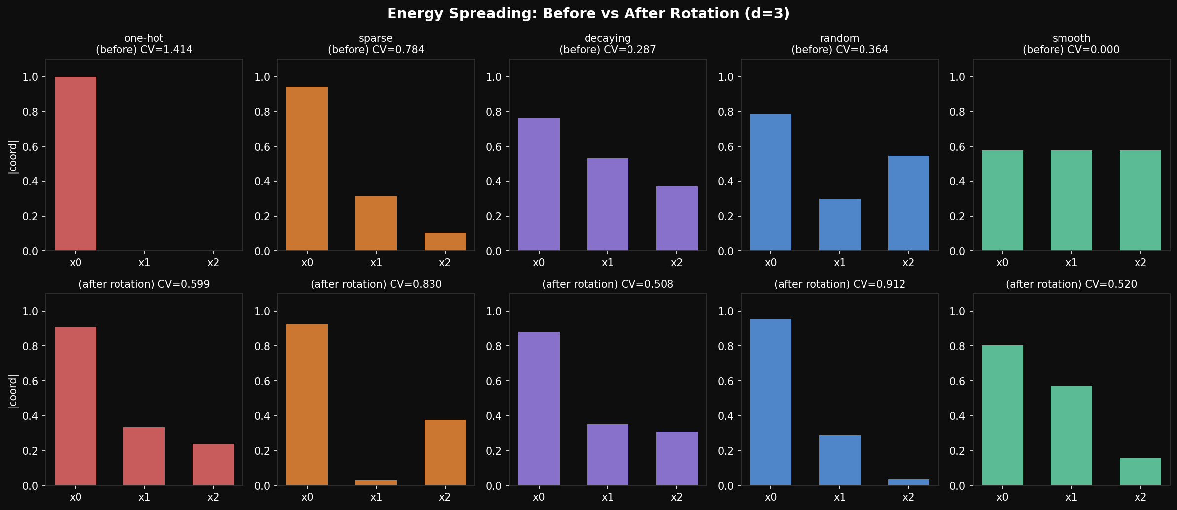 Energy spreading illustrated in d=3 for visual clarity.
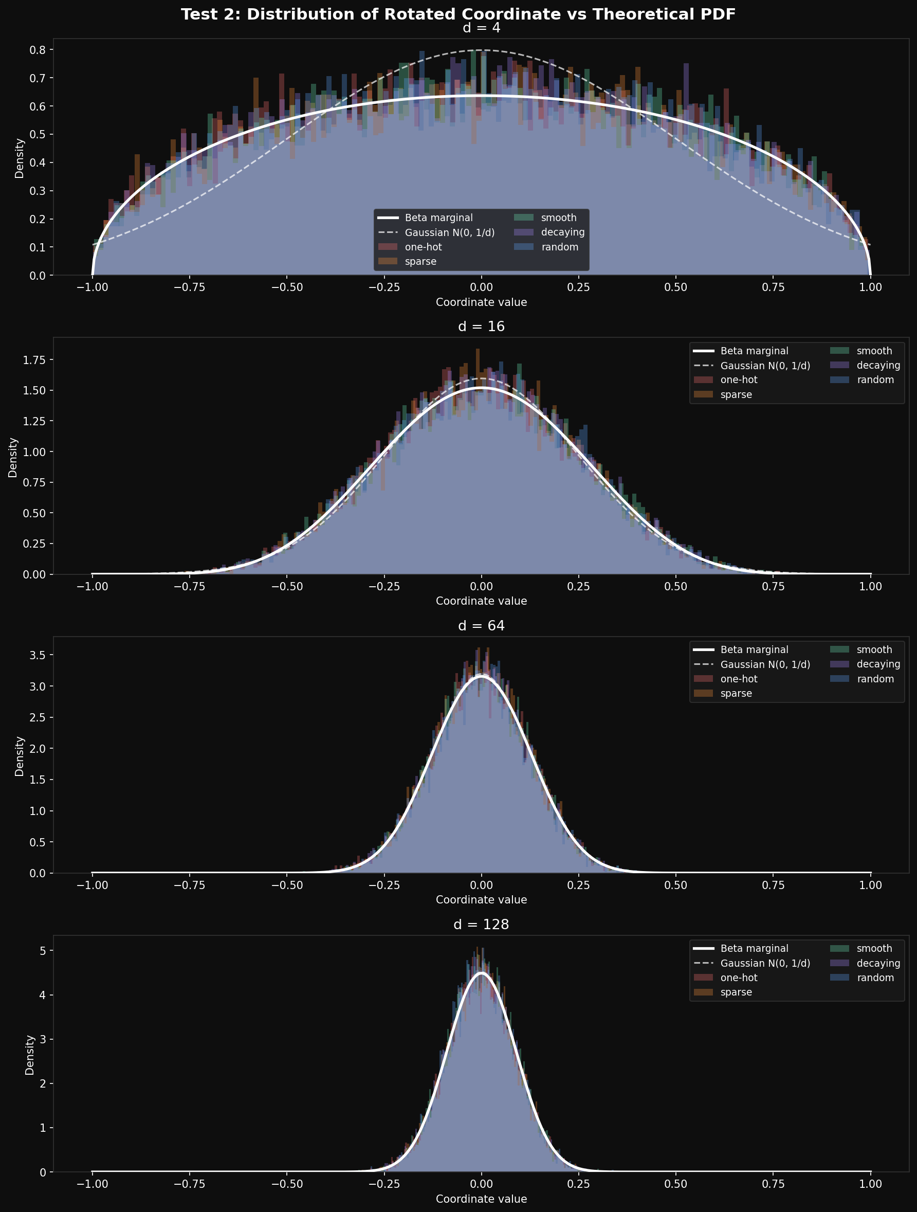 Empirical distribution of rotated coordinates vs. theoretical Beta/Gaussian fit.
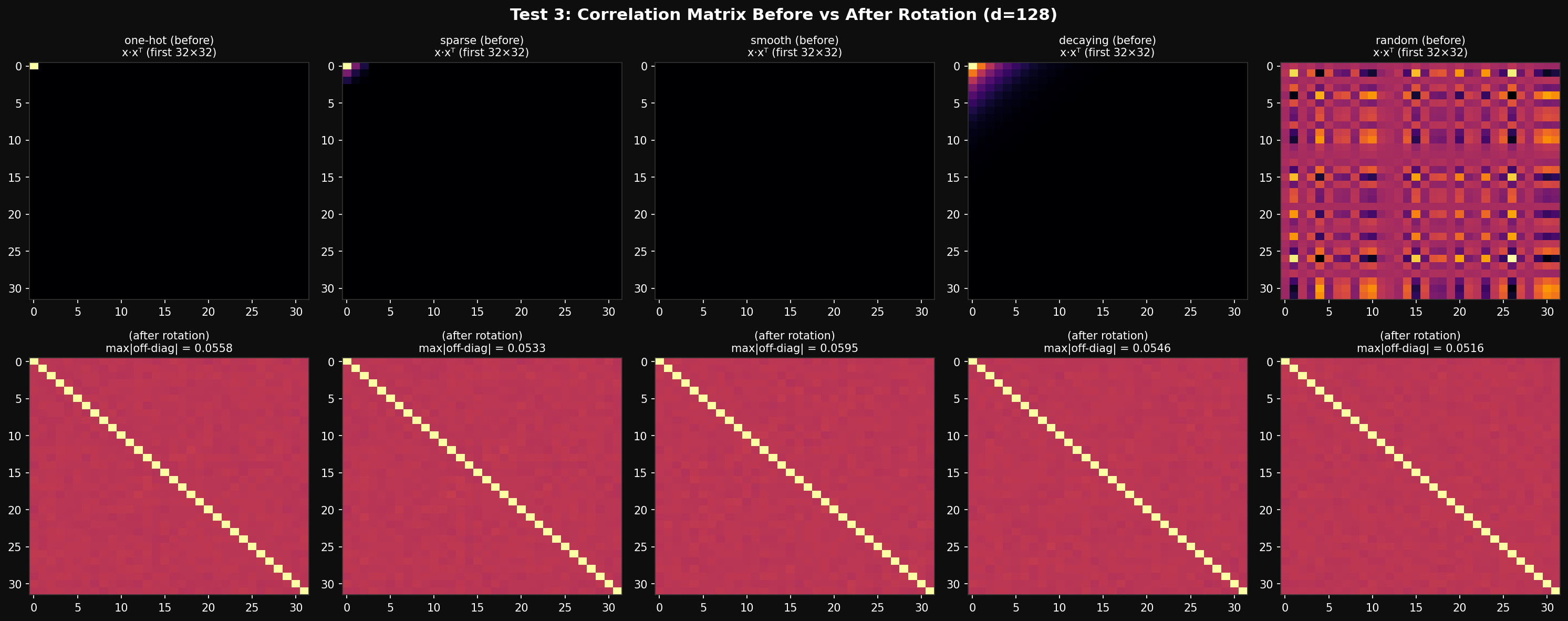 Pair-wise correlation of coordinates after rotation — near-zero off-diagonal entries confirm near-independence.
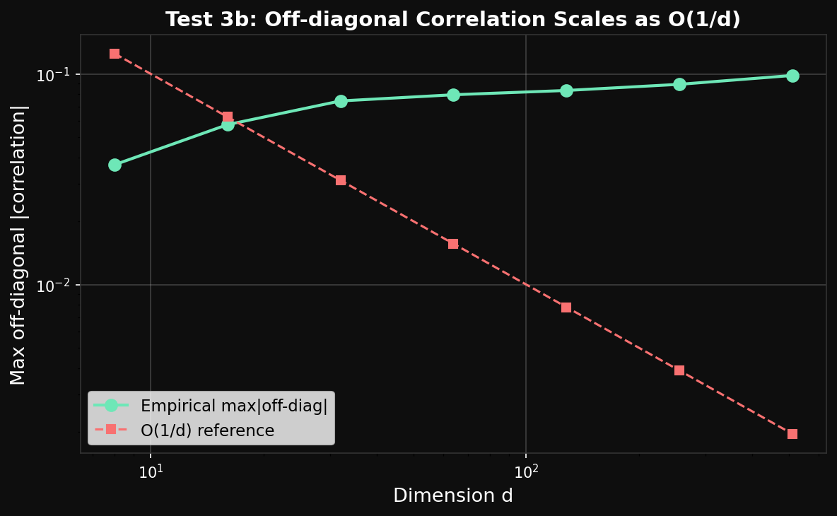 Off-diagonal correlation decays as d increases, validating the independence assumption.
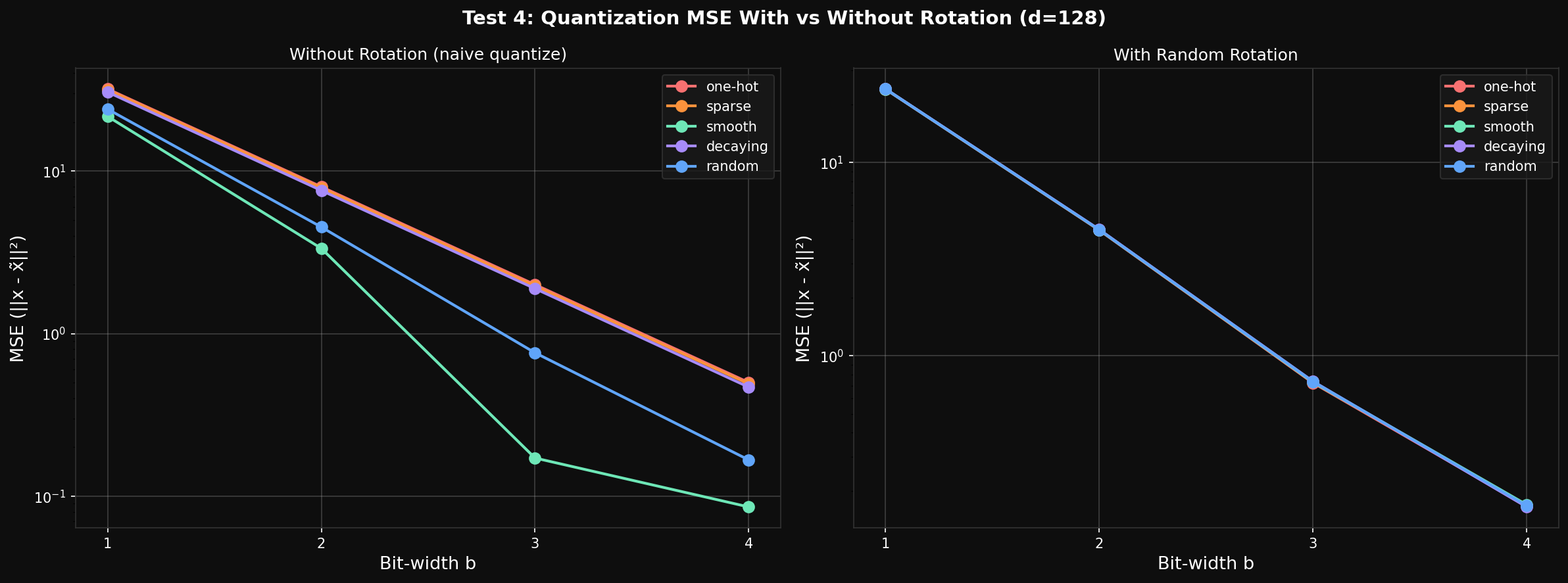 Empirical MSE vs theoretical upper and lower bounds across bit-widths b=1..4 on synthetic unit vectors.
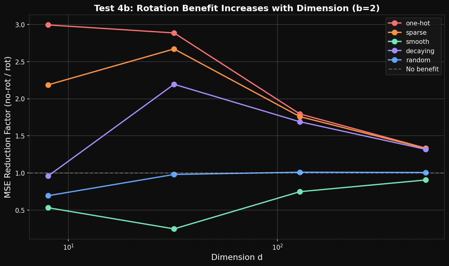 MSE as a function of dimension d — confirms the distortion-rate bound scales correctly with d.
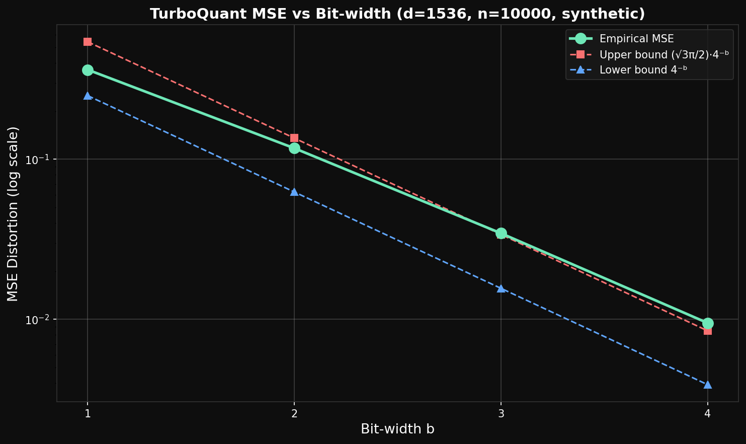 Reproduction of Fig. 3 on synthetic data: empirical MSE lies between Shannon lower bound (1/4^b) and TurboQuant upper bound (√3π/2 · 4^(-b)).
Phase 2 — GloVe 300d
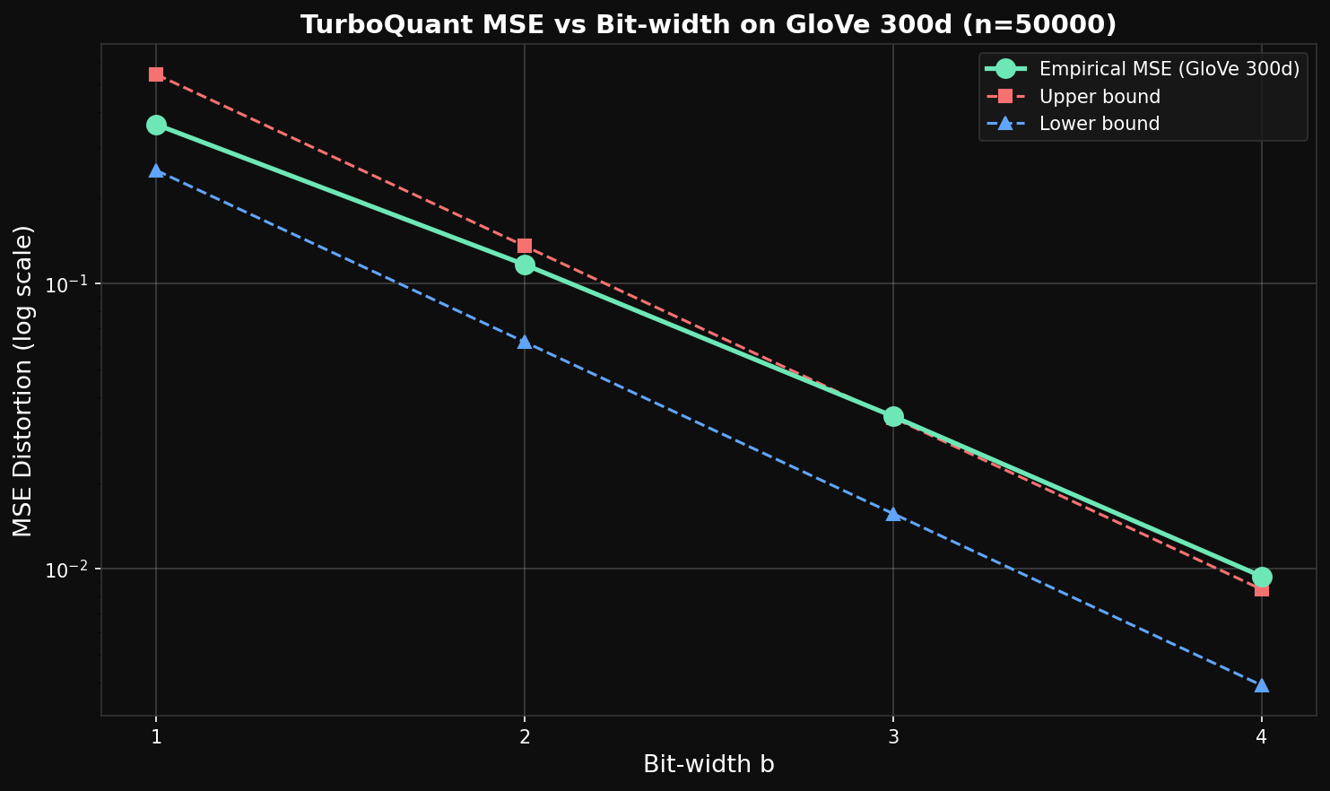 Empirical MSE on GloVe 300d embeddings vs theoretical bounds for b=1..4. Confirms the algorithm works on real-world non-unit-sphere data.
Phase 3 — DBpedia 1536d (Paper Figures)
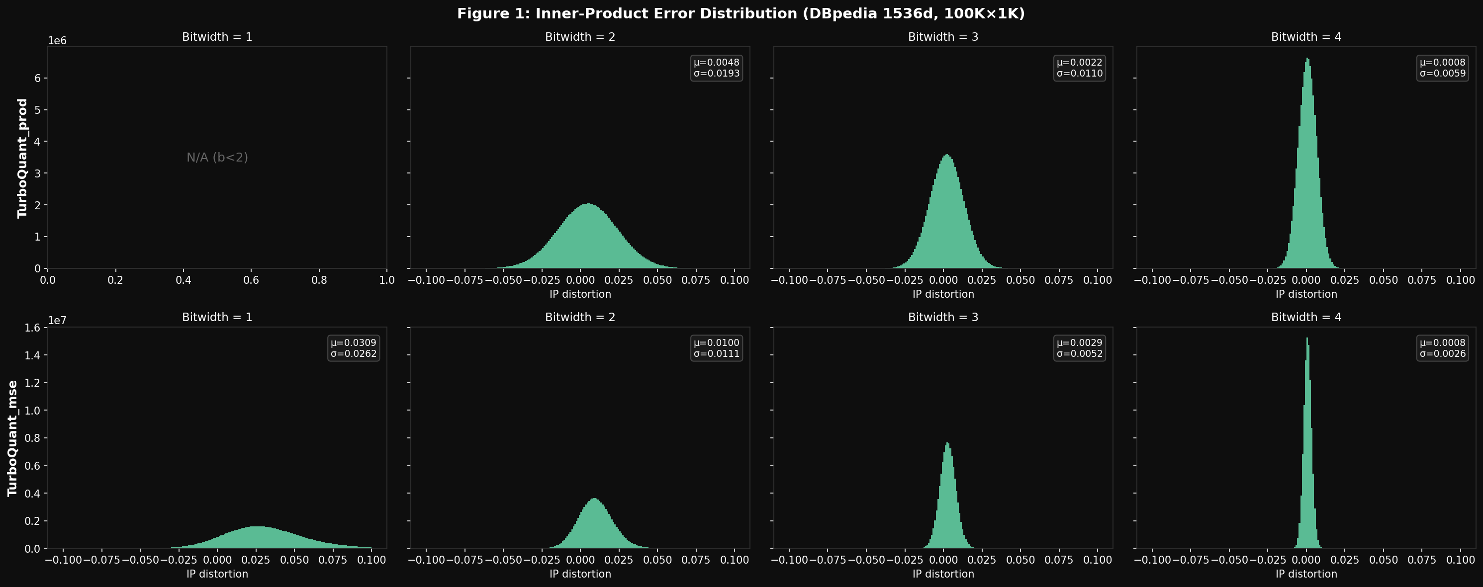 Fig. 1 reproduction: inner-product error histograms for TurboQuant_prod (top) and TurboQuant_mse (bottom) at b=1,2,3,4. prod remains unbiased (centered at 0); mse shows rightward shift at low bit-widths. Passing criteria: Both quantizers must produce roughly Gaussian error distributions, and variance must shrink with increasing bitwidth.
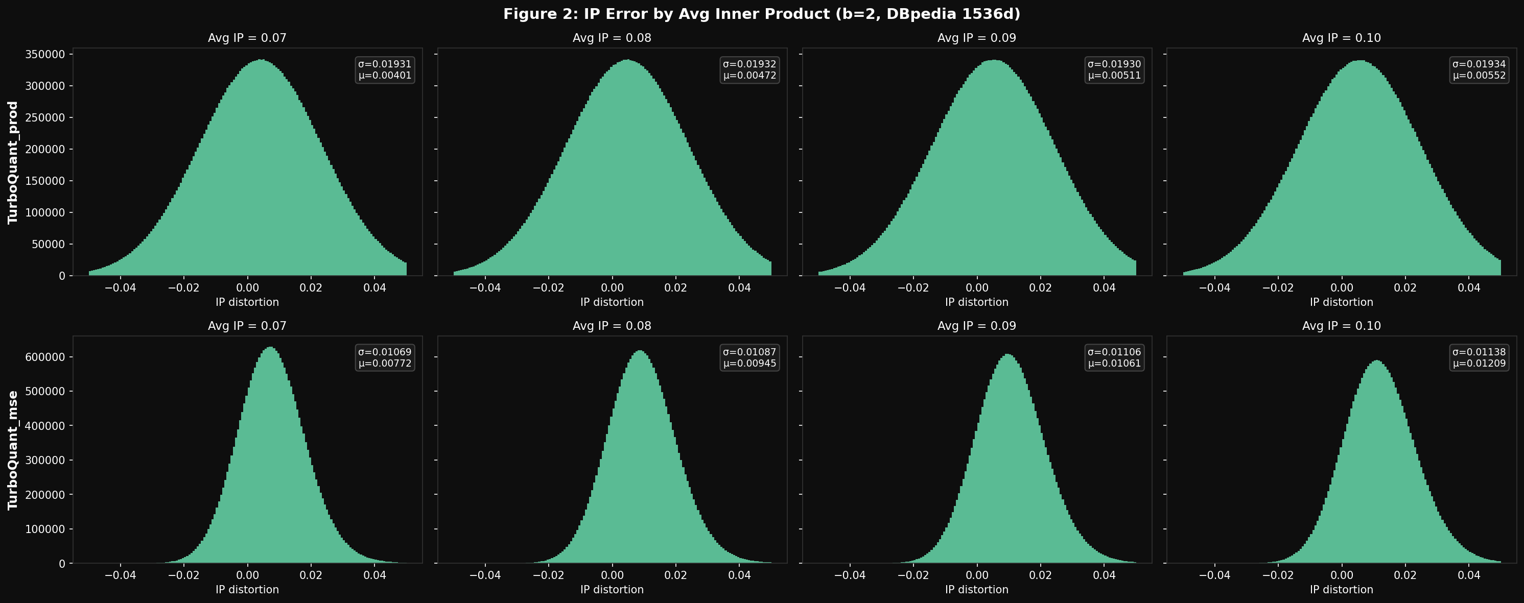 Fig. 2 reproduction: inner-product error histograms at b=2, grouped by average inner product of each database vector. prod variance is constant across groups; mse variance grows with average inner product. Passing criteria (core theoretical claim): TurboQuant_prod histogram width must stay constant across all avg IP values (variance independent of inner product magnitude); TurboQuant_mse histogram must get wider as avg IP grows. If both rows look the same, the QJL residual correction is not working.
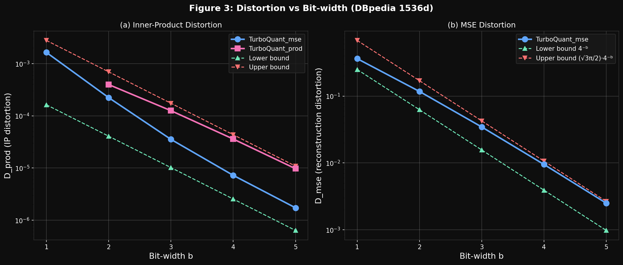 Fig. 3 reproduction: empirical D_prod and D_mse vs bit-width b=1..5 on DBpedia 1536d. Both curves lie between theoretical bounds (dashed). At b=1, TurboQuant_mse exceeds the inner-product upper bound — expected, since it is biased for inner products at low bit-widths. Passing criteria: Empirical MSE must fall between the paper’s upper and lower bounds.